Object Detection의 subtask인 Face Detection 연구 중 하나로, 2019년 발표된 논문이다. extra supervision (label을 손수 추가)과 self supervision을 joint하게 학습시킴(multi-task learning)으로써 WIDER FACE hard 데이터셋 기준 기존 SOTA보다 1.1% 정도의 face box AP를 끌어올렸다.
RetinaFace

WIDER FACE hard test set → 91.4%로 기존 SOTA보다 1.1% 앞섬.
IJB-C test set, RetinaFace을 사용하면 face verification의 sota인 ArcFace도 성능 향상이 이루어짐
Backbone을 가볍게 한다면 싱글 코어 CPU 환경에서도 실시간으로 수행이 가능함.
How? joint extra-supervised and self-supervised multi-task learning→ 이걸 병렬적으로 구성해서 multi-task한다는 건 output을 아예 여러 개 내뱉는다는 거. (아래처럼)

existing branch
- 기존의 일반적인 detection network (classification과 box regression의 multi-task learning 구조)
extra-supervision branch
- retinanet에서는 5개의 face landmark annotation을 추가해줌. (extra label이 추가 → extra-supervision)
- 이를 regression하는 branch가 extra-supervision branch
self-supervision (self-supervised mesh decoder branch)
- pixel-wise 3D shape face information을 예측, 해당 브랜치는 supervised branch와 병렬적으로 구성
- a.k.a. dense regression branch (pixel-wise localization)
- colored face mesh를 하나의 그래프 $\mathcal{G} = (\mathcal{V},\mathcal{E})$ 로 정의함.
- 이때 $\mathcal{V}$는 joint shape and texture information을 담는 face vertices의 집합임 (n*6 차원의 실수집합에 속함)
- → a joint shape and texture decoder
- Edge $\mathcal{E}$는 vertices 간 연결여부를 나타내는 $n \times n$ sparse 인접행렬로 구현됨.
- graph convolution $g_\theta$ 의 수식은 다음과 같이 정의됨.
- $L = D-\mathcal{E}$ ($L$ : graph Laplacian)
- 이때 $D$는 그래프 차수로, $n\times n$ 의 대각행렬
- recursive Chebyshev polynomial truncated at order K의 형태로 formulated
- $\theta$: K-dim의 체비셰프 계수 벡터
- $T_k(\tilde{L})$: scaled Laplacian $\tilde{L}$에서 계산되는 k차 체비셰프 다항식 (nxn)
- 위의 식을 풀면, $[\bar{x}_0, ..., \bar{x}_{K-1}]\theta$ 의 형태로 reduce됨. 이때, $\bar{x}_k = T_k(\tilde{L})x$ 임.
- 점화식 형태($\bar{x}_k = 2\tilde{L}\bar{x}_{k-1} - \bar{x}_{k-2}$, $\bar{x}_0 = x\ and\ \bar{x}_1 = \tilde{L}_x$)로 계산되고, 위의 filtering 연산은 굉장히 효율적. (due to K sparse matrix-vector multiplications and one dense matrix-vector multiplication)
- cf.) graph convolution
- 2D convolution operation → kernel-weighted neighbor sum within the Euclidean grid receptive field
- 둘 다 kernel-weighted neighbor sum이라는 개념은 같음.
- 2d conv의 경우에는 kernel size로 neighbor를 정의하지만, graph conv에서는 두 정점을 잇는 edge의 최소 개수를 count하는 형식으로 neighbor distance를 정의함.
- 이 경우에는 parameter 개수가 $K\times Channel_{in} \times Channel_{out}$

- 이 경우에는 parameter 개수가 $K\times Channel_{in} \times Channel_{out}$
- $L = D-\mathcal{E}$ ($L$ : graph Laplacian)
- $$y = g_\theta(L)x = \sum_{k=0}^{K-1}\theta_kT_k(\tilde{L})x$$
- Differentiable Renderer
- mesh decoder는 3D mesh를 predict해줌. 하지만 우리의 target은 2D 이미지 상에 존재. 따라서 3D to 2D로 projection해줘야함.
- colored mesh $\mathcal{D}_{P_{ST}}$ to be projected onto a 2D image plane with camera parameters $P_{cam} = [x_c, y_c, z_c, x'_c, y'_c, z'_c, f_c]$ (i.e. camera location, camera pose and focal length) and illumination parameters $P_{ill} = [x_l, y_l, z_l, r_l, g_l, b_l, r_a, g_a, b_a]$ (i.e. location of point light source, color values and color of ambient lighting)
- $P_{ST}$ → shape and texture parameters (128차원의 실수집합 내에 존재)
- Dense Regression Loss (pixel-wise)
- $W$, $H$ : the width and height of the anchor crop $I^*_{i,j}$, respectively
- $$L_{pixel} = \frac{1}{W*H}\sum_{i}^{W}\sum_{j}^{H}\Vert\mathcal{R}(\mathcal{D}_{P_{ST}},P_{cam},P_{ill})_{i,j} - I^*_{i,j}\Vert_1$$
- mesh decoder로 graph convolution (based on fast localized spectral filtering) 을 이용.
output = (bbox_out, cls_out, landmark_out, mesh_out)→ 총 3가지의 branch가 있음. (in parallel)
Context Module
- 마치 FCN에서 decoding할 때 (upsampling), skip connection 더해준 거처럼 각 feature pyramid마다 넣어주기..
ablation study
- dense regression은 추가하면 오히려 hard의 경우는 boxAP가 하락함.
- 반면, landmark branch의 추가는 모든 경우에 다 성능 향상을 가져옴
- dense regression과 landmark를 두 개 다 추가해주면, 가장 성능이 좋았음. (landmark detection이 dense regression task를 도와줌을 알 수 있음)

Inference Efficiency
- lightweight version을 사용해서 inference 속도를 높이겠다.
- lightweight, 즉 MobileNet-0.25 backbone을 사용하는 경우 AP 78.2% on WIDER FACE hard set
- light-weight의 경우에는, 7x7 conv (stride of 4)를 사용해서 이미지를 빠르게 축소시켜줌. deformable layers는 없애줌.
- 처음 두 개 conv layer는 높은 accuracy를 달성하기 위해 ImageNet에서 사전학습된 weight으로 고정해줌.
- inference time 비교
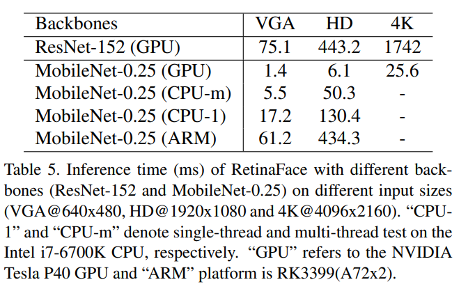
- VGA(640X480)의 경우, single-thread cpu에서 60fps, ARM에서는 16fps의 속도를 보여줌. (모바일에서도 어느 정도 빠른 구동이 가능하다)
notion에 적어뒀던 걸 옮기느라 가독성이 조금 떨어지는 듯하다. ㅠㅠ
'DeepLearning > Computer Vision' 카테고리의 다른 글
| [Generative Models] Unpaired Image-to-Image Translation using Cycle-Consistent Adversarial Networks (2017) (1) | 2022.04.17 |
|---|---|
| [Generative Models] Unsupervised Representation Learning With Deep Convolutional Generative Adversarial Networks (2016) (3) | 2022.04.15 |
| [CV] OCR의 data format (1) | 2021.11.10 |
| [CV] OCR - 글자 영역 검출 (0) | 2021.11.09 |
| [Object Detection] Focal Loss (0) | 2021.09.30 |