Faster R-CNN
: Towards Real-Time Object Detection with Region Proposal Networks

Idea
Fast R-CNN은 selective search 수행으로 인한 region proposals(object가 있는 곳을 파악하는 과정)에서의 시간 소요 (bottleneck)가 단점으로 작용함
Faster R-CNN에서는 Region Proposals를 CNN으로 수행함으로써 속도 개선 (“Region Proposal Networks; RPNs” )
→ end-to-end object detection model 구성
→ 5 fps 까지의 속도 향상, Pascal VOC 기준 mAP 78.8%의 성능 개선
RPNs

- Region proposals 부분에서 selective search 대신 Fully Connected CNN(RPN)을 통해 RoI (Region of Interest)를 계산함.
- 이후 Fast R-CNN과 convolutional layers를 공유하게끔 디자인되어 있음.
- CNN으로 구조 변경을 통해 GPU를 통한 RoI 계산이 가능해짐. (병렬화로 인한 speed up)
- 다양한 크기의 이미지를 입력받아 Object(Rectangular regions) Proposal과 Objectness Score(“Objectness” measures membership to a set of object classes vs. background.)를 출력
Anchor box
- Anchor Box: Sliding Window의 각 위치에서 Bounding Box의 후보로 사용되는 상자.
- 기존에는 이미지 크기를 조정하거나(image/feature pyramids) 혹은 filter size를 조정(pyramids of filters)하는 방식으로 다양한 크기와 비율의 Sliding Window를 사용하여 region proposals을 수행.
- RPNs에서는 하나의 Sliding Window 크기를 사용하며, 이를 위해 다양한 크기와 비율의 Anchor Box가 동원되는 형식으로 보다 효율적.
- 논문에서는 3가지 크기, 3가지 비율 총 9가지의 anchor box 사용.
- Translation-Invariant, which also reduces the model size. (lower risk of overfitting on smaller datasets)
How it works
- CNN을 통해 뽑아낸 feature map(H, W, C) 을 입력으로 받음
- 1의 피처 맵을 대상으로 n=3인 nXn convolution을 수행 (output channel dim: 256 or 512-d) à 이때 output의 크기를 동일하게 하기 위해 padding을 진행
- 2에서 얻은 피처 맵을 각각 2개의 FC layers로 보내줌 (box-regression layer and box-classification layer), 정확히는 FC layer가 1X1 convolution 형식으로 구현
- Classification – 2*9 필터 수만큼 1X1 conv (2: 물체인지 아닌지 나타내는 index 수, 9: 앵커 개수) à (H,W,18) 리턴.
- Regression – 1X1 conv filters (4*9=36개) (4: dx,dy,w,h의 박스 좌표 표시를 위한 데이터, 9: 앵커 개수) à (H,W,36) 리턴.
cf.) RPN에서의 라벨 값 할당
- 두 개의 label 값 (object or not)
- positive label의 할당 기준 (물체라고 판단하는 기준)
1) 가장 높은 Intersection-over-Union (IoU)를 가지고 있는 anchor
2) IoU > 0.7을 만족하는 anchor
2)를 우선적으로 고려하고, 2)를 모든 anchor가 만족하지 못할 시에 1)의 기준을 적용한다.
Multi-task Loss Function
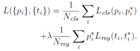
multi-task loss로, classification task와 regression task에 대한 loss가 결합되어 있는 형태이다. 앞부분은 classification task, 뒷부분은 regression task에 대한 loss이다.
- $p_i$: predicted probability of anchor
- $p_i^*$: Ground-truth label (1: positive, 0: negative)
- $t_i$: predicted bounding box
- $t_i^*$: Ground-truth box
- $N_{cls}$: classification task에 대한 미니배치 크기
- $N_{reg}$: regression task에 대한 미니배치 크기
- $\lambda$: Balancing Parameter. $N_cls$와 $N_reg$ 차이로 발생하는 불균형을 방지. $N_cls$가 256이고, 이미지 내부에서 사용된 모든 anchor의 location($N_reg$)이 약 2400이라고 가정하면 $\lambda$는 대략 10으로 설정
[$t_i$ 계산식]

$x, y, w, h$는 box의 offsets (각각 box의 중심 좌표와 너비, 높이를 나타냄).
[regression loss]

regression loss는 smooth L1 loss를 사용함.
classifcation loss는 log loss (binary classification: object가 box 내에 존재하는가 여부)를 사용한다.
Training
Alternative Training
Fast R-CNN과 연결하여 학습시키기 위해 4단계에 걸쳐서 모델을 번갈아서 학습
- Load pre-trained model and train RPNs
- Train Fast R-CNN using the proposals from RPNs (기본 CNN 제외)
- Fix the shared convolutional layers and fine-tune unique layers to RPNs
- Fine-tune unique layers to Fast R-CNN
→ 학습과정이 다소 복잡함. 추후 joint training 기법을 활용하여 개선.
Training details
- SGD로 최적화
- anchor의 경우 negative, positive를 각각 1:1비율로 하여 256개 랜덤 샘플링
($\because$ negative example로 편향될 가능성 O) - mean = 0, sd = .01의 정규분포로 weight random init
- learning rate = .001(처음 6만개 미니 배치), 이후 .0001로 감소시킴
- Momentum = .9
- Weight Decay = .0005
'DeepLearning > Computer Vision' 카테고리의 다른 글
| [Object Detection] Focal Loss (0) | 2021.09.30 |
|---|---|
| [DL/CV] NN interpolation의 backward propagation (0) | 2021.09.29 |
| [Object Detection] Image Annotation Formats (0) | 2021.03.17 |
| [Object Detection] object detection 성능평가지표 (2) | 2021.03.03 |
| [Object Detection] RefineDet 리뷰 (0) | 2021.03.01 |